
In last week’s post I set out the premise behind our choice to use Citizen Science for exploring our LiDAR survey, and started to look at some of the statistics we have generated from the portal with regard to patterns of use. We’ve had quite an exciting week here at Hillfort Towers, with a nice write-up in The Times on Wednesday (paywall) along with the University of Exeter’s Understanding Landscapes Project. (Of course this means all my carefully crafted stats are horribly out of date, with a record-breaking 92 new users registering on Wednesday, and 108 unique users logging in!) So welcome to all the new users.
Let’s continue our analysis of some of the data you’ve been generating. The first thing to look back at are the user stats – I had some fun taking the anonymised IP addresses and plotting those on a map to see where (very generally and imprecisely, to town/city level – don’t worry, we’re not spying on you) you are signing in from… turns out we’ve got a pretty good spread across the (English-speaking) world! Click here, or on the map below, and see if you can spot yourself…!
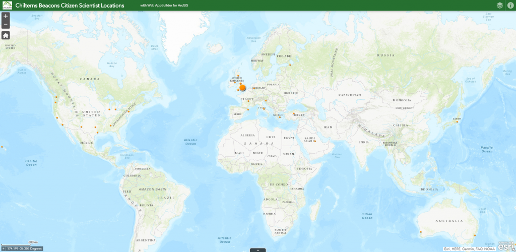
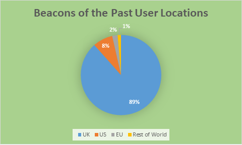
Roughly 35% of you are within 5 km of the survey area – perhaps not that surprising. In total 89% of you are in the UK, with around 8% of users being in the USA (including one person in Hawaii!), just 2% in the EU, and around 1% across the rest of the world, including countries such as Russia, Saudi Arabia, Turkey, Japan, Australia, and New Zealand.
Our fantastic global user base has created around eight and a half thousand “Citizen Records” now! Let’s have a bit of a look at the patterns emerging from them – data correct as of 6th May 2020.
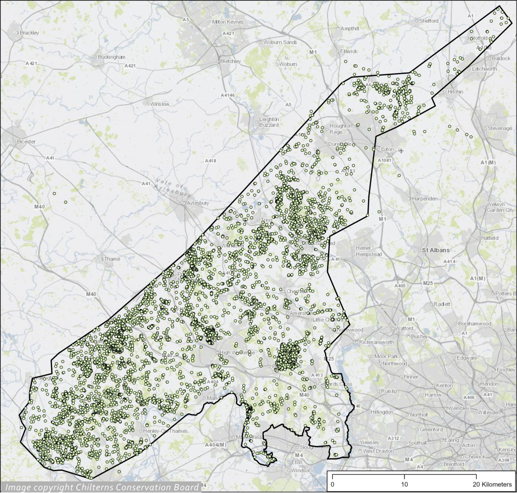
Contains OS data © Crown copyright and database right (2020)
The distribution across the survey area is, as you might expect, not particularly even, with certain “hot spots” where users have focused their recording. The map above with simple dots (“centroids” of Citizen record polygons) gives some idea of that distribution. The overlapping dots are not particularly easy to see though, so instead we can use a statistical technique called “kernel density” plotting to generate a type of “heat map” to show the relativey local density patterns a bit more clearly.
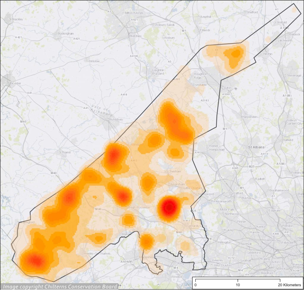
Image copyright CCB. Contains OS data © Crown copyright and database right (2020)
We can see several foci in the data. The strongest focus of records is in the vicinity of Chalfont St Giles, centred on a piece of woodland called Hodgemoor Woods. We can see a more or less continuous focus of records along the Oxfordshire stetch of the escarpment slope and just into Buckinghamshire, roughly between the Goring Gap and Wendover, but with special hot spots along there around Goring Heath parish, around Christmas Common, and above Princes Risborough. The foci north of High Wycombe are on the National Trust properties of Hughenden and Bradenham; the blob north of Maidenhead is the Cliveden Estate. The Bulbourne Valley, around Berkhamstead and onto the Ashridge Estate, has also seen lots of records, and in the northern Chilterns the Sundon and Barton Hills form the focus of work up there.
So what drives these patterns? There are two core reasons I think. The primary reason is this is a pattern reflecting where people have spent time looking and recording: I know that just a handful of individuals might be responsible for some of these densities, for example along the Oxfordshire escarpment, or in Hodgemoor Woods where individuals have put in lots of time and energy to mapping the features in a particular area (our top 5 most prolific recorders have, between them, recorded an astonishing 4500 sites!). Individuals and groups of National Trust volunteers have put in lots of hard work mapping what can be seen across those properties, and similarly a team of members of South Oxfordshire Archaeology Group have been working on a parish-based study of Goring Heath, explaining the density of records there. So rather than being a pattern of where the archaeology is, this general overview shows a pattern of where our Citizen Scientists have been focusing their efforts.
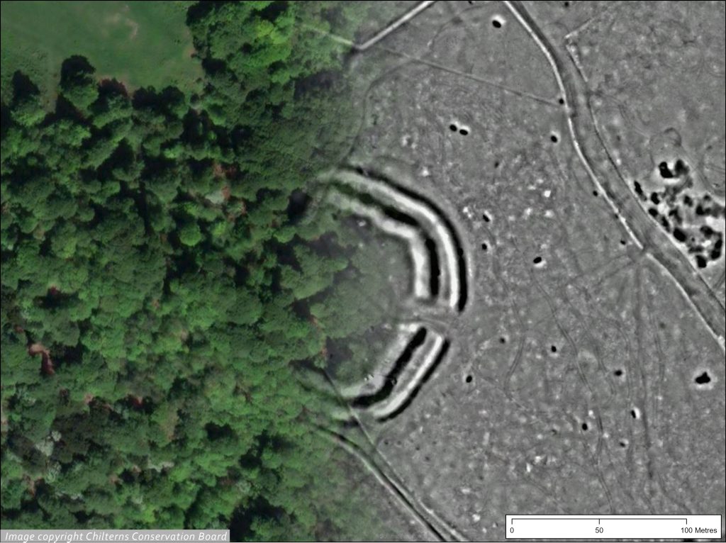
hiding in woodland, and revealed by LiDAR. Image copyright CCB. Contains aerial imagery
© Getmapping Plc and Bluesky International Limited (2020)
However, these is of course the possibility that other patterns lie in these data: where monuments were preferentially created, and where monuments survive to be detected in LiDAR. The former is I think very difficult to identify, but the latter I think we can certainly see in this pattern: 39% of the 8,300 odd records lie within woodland recorded as Ancient Woodland by Natural England, by which it means land which has been wooded since 1600 or before. There are only 215 square kilometres of ancient woodland in the survey area, meaning that 39% of our records fall into just 15% of the area! Earthworks which lie on land which has been continuously wooded through the post medieval period are far more likely to survive, not being subject to the threats of the plough or the developer. I think there is much more work to be done to test this and other patterns in the data, but suffice to say that our woodlands are yielding fantastic new archaeological stories.
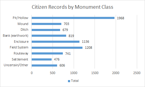
Finally, a quick look at the data on what types of monument are being found. Obviously some individual sites are likely to have been duplicated in these data… lots of people have drawn around the hillforts, for example. By far in a way the leaders though are “pits/hollows”, reflecting something I often say in talks on the LiDAR… the Chilterns are full of holes! You can find chalk pits, clay pits, saw pits, and other assorted “divots” across the whole study area.
Field systems are second in the list – this may of course reflect that the majority of the landscape is farmed, so covered in modern and older fields; this also reflects one of the more exciting new narratives that this LiDAR survey is able to show – the subtle but distinct traces of extensive later prehistoric or Roman field systems hiding in many patches of woodland, something which wasn’t generally known before, as they are so difficult to spot on the ground.
Enclosures come next, I think not because of their frequency (although we certainly do have some exciting new sites showing up), but perhaps more because of their distinctiveness and the interest that they draw.
I think that will conclude our little exploration of some of the data for now… there’s plenty more to say, so let me know in a comment below if there are any particular topics you want me to discuss!
Hi Ed,
I was one of those who joined after reading the Times article. I am doing the tutorials and have had a look over the maps and Lidar information. I live in Rutland but do drive through it occasionally, so can appreciate the work that the project has undertaken.
I was doing the footpath surveys with the Ramblers, but this is far more complicated – trying to get to grips with the various monuments will be a challenge for a while.
The Ramblers survey used a grid system based on the OS maps, so could you use a similar system so that those of us who do not know the area can concentrate on ‘less popular’ areas?
Regards,
Glyn
Great work so far Ed. Not that I’m biased in any way!